Analyzing Sleep Patterns with the Oura Ring

In the year 2023 I made the decision – I am going to get better sleep. I went ahead and purchased an Oura ring (https://ouraring.com/oura-experience). While the ring itself was uncomfortable at first, I was amazed at the data exploration possibilities I saw even in the first week. Eventually the discomfort of a bulky ring dissipated and was replaced with the excitement of gaining new insights into my sleep habits.

The personal data can be downloaded through a user’s account on Oura as a csv. In my analysis, I used Python and Tableau for cleaning and visualizing the data. My goals were to create a dashboard with a filter on time so I could see how my sleep habits changed over the year and to gain a greater understanding of what goes into the all important Sleep Score that is calculated when I sync every morning.

Initial Cleaning

In order to get a clean data set, I first had to find any missing data and add any features that may be useful. I was anxious to get started so I used a go-to tool for when I want to get started quickly – Google Colab. Its clean interface and quick startup made it an obvious choice for this project. The csv is loaded into a DataFrame format and the info is shown below. An initial look at my data showed 55 columns – only some of which were of particular interest to me. In order to make the data more useful, I needed to add some new features or clean up existing columns.

RangeIndex: 356 entries, 0 to 355

Data columns (total 55 columns):

#	Column	Non-Null Count	Dtypes
---	------	-----------------	------
0	date	356 non-null	datetime64[ns]
1	Sleep Score	355 non-null	float64
2	Total Sleep Score	355 non-null	float64
3	REM Sleep Score	355 non-null	float64
4	Deep Sleep Score	355 non-null	float64
5	Sleep Efficiency Score	355 non-null	float64
6	Restfulness Score	355 non-null	float64
7	Sleep Latency Score	355 non-null	float64
8	Sleep Timin Score	355 non-null	float64
9	Total Sleep Duration	355 non-null	float64
10	Total Bedtime	355 non-null	float64
11	Awake Time	355 non-null	float64
12	REM Sleep Duration	355 non-null	float64
13	Light Sleep Duration	355 non-null	float64
14	Deep Sleep Duration	355 non-null	float64
15	Restless Sleep	355 non-null	float64
16	Sleep Efficiency	355 non-null	float64
17	Sleep Latency	355 non-null	float64
18	Sleep Timing	355 non-null	float64
19	Bedtime Start	355 non-null	object
20	Bedtime End	355 non-null	object
21	Average Resting Heart Rate	355 non-null	float64
22	Lowest Resting Heart Rate	355 non-null	float64
23	Average HRV	355 non-null	float64
24	Temperature Deviation (°C)	355 non-null	float64
25	Temperature Trend Deviation	355 non-null	object
26	Respiratory Rate	355 non-null	float64
27	Activity Score	356 non-null	object
28	Stay Active Score	356 non-null	object
29	Move Every Hour Score	356 non-null	object
30	Meet Daily Targets Score	356 non-null	object
31	Training Frequency Score	356 non-null	object
32	Training Volume Score	356 non-null	object
33	Activity Burn	356 non-null	int64
34	Total Burn	356 non-null	int64
35	Steps	356 non-null	int64
36	Equivalent Walking Distance	356 non-null	int64
37	Inactive Time	356 non-null	int64
38	Rest Time	356 non-null	int64
39	Low Activity Time	356 non-null	int64
40	Medium Activity Time	356 non-null	int64
41	High Activity Time	356 non-null	int64
42	Non-wear Time	356 non-null	int64
43	Average MET	356 non-null	float64
44	Long Periods of Inactivity	356 non-null	int64
45	Readiness Score	355 non-null	float64
46	Previous Night Score	355 non-null	object
47	Sleep Balance Score	355 non-null	object
48	Previous Day Activity Score	355 non-null	object
49	Activity Balance Score	355 non-null	object
50	Temperature Score	355 non-null	float64
51	Resting Heart Rate Score	355 non-null	object
52	HRV Balance Score	355 non-null	object
53	Recovery Index Score	355 non-null	float64
54	Sleeping Hours	355 non-null	float64

dtypes: datetime64[ns](1), float64(28), int64(11), object(15)

memory usage: 153.1+ KB

Simplest among typical cleanup tasks is converting any time features to datetime. From here, it is possible to easily break out the date objects (year, month, day) for ease of use in further analysis.

data['date'] = pd.to_datetime(data['date'])

data['Bedtime Start'] = pd.to_datetime(data['Bedtime Start'])

data['Bedtime End'] = pd.to_datetime(data['Bedtime End'])

data['day'] = data['date'].dt.day

data['month'] = data['date'].dt.month

data['year'] = data['date'].dt.year

It is also possible to change the data type in Tableau by right clicking on the measure in the Data panel and selecting “Date & Time” under “Change Data Type”. When moved into the columns or rows, it can be broken down further into the date objects easily.

Oura reports time in seconds, where it is much clearer to review in hours, so all duration related columns were converted to hours.

#convert seconds to hours

data['Sleeping Hours'] = data['Total Sleep Duration']/3600

data['REM Sleep Duration'] = data['REM Sleep Duration']/3600

data['Light Sleep Duration'] = data['Light Sleep Duration']/3600

data['Deep Sleep Duration'] = data['Deep Sleep Duration']/3600

This is not a very large dataset, so cleanup was fairly simple. Oura did add certain features over the course of the year so there were some null values under those columns but they were disregarded for the purposes of this study.

Visualization

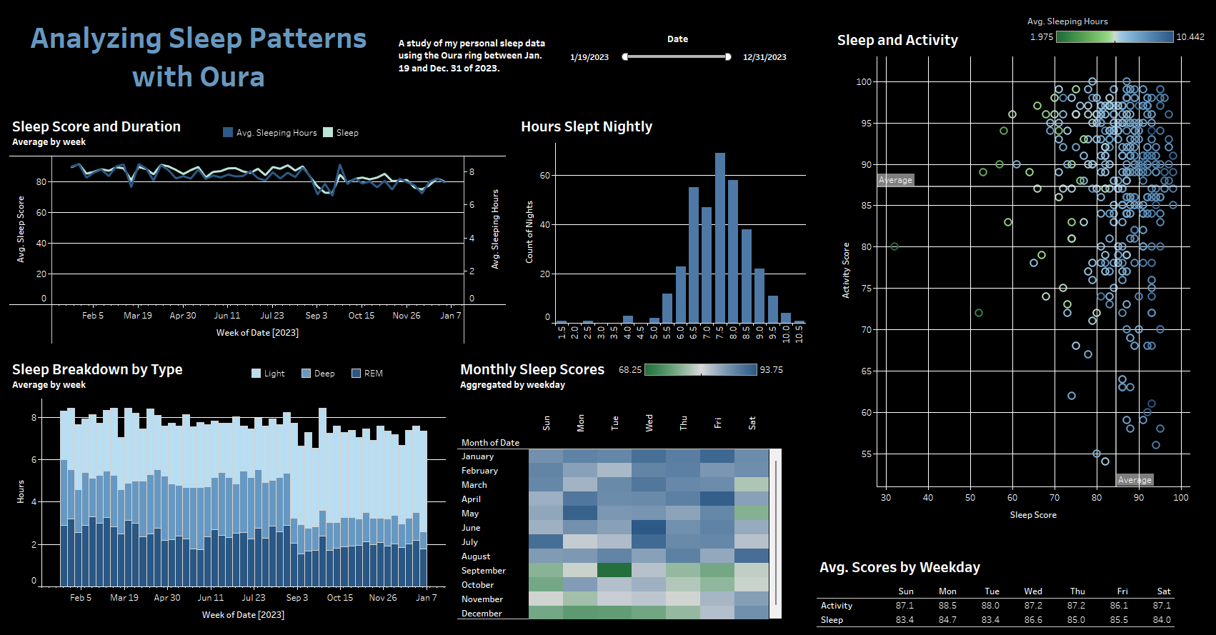
I wished to create a dashboard to track how my sleep habits changed over the year. On my list of requirements was the ability to zoom in on certain time periods over the year where I knew I had changes to my normal routine. I also wanted to see a distribution of my total hours slept over the course of the year, get an understanding of whether the days of the week had any impact on sleep or activity, and see the general trends over time.

I played around with using Matplotlib and Seaborn to get some initial ideas for my visualizations, but for the dashboard creation I chose to complete the task in Tableau. Additional benefits of using Tableau for this task include a clean overall look, ease of sharing online, and interactive filters without using additional packages such as Plotly.

I created this dashboard keeping principles learned in my Google Business Intelligence Certificate in mind.

Some additional visualizations that I did not determine needed inclusion in my dashboard follow.

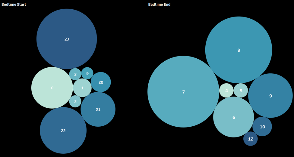
Packed bubbles are a nice visualization for a quick overview of the general patterns found in the data. However, when you get close numbers, such as the hours of 7 AM and 8 AM on the Bedtime End plot, you cannot tell which is the larger of the two at first glance. Here, the tooltip is useful to display the counts or the preferred plot may be a histogram.

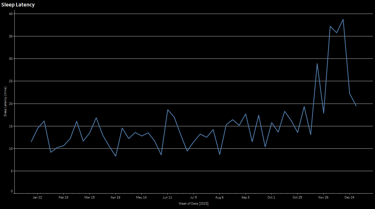
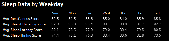
I did want to see some more on the factors contributing to Sleep Score (see Modeling section for more) but I felt the figures did not truly contribute to the overall story in a meaningful way. I chose to use a line plot to look at sleep latency (how long it takes to fall asleep) averaged weekly over time and a text table to look at several of the scores.

Analysis

Some immediate insights from my dashboard include that I had a slight drop in the summer in my sleep scores, more than likely due to having an old house with a lack of air conditioning.

In early September I went to a wedding in California. It was my first time leaving the Eastern time zone and it was clearly reflected in my sleep (see average weekly scores). I must be high maintenance because for the next several weeks, my sleep scores did not recover! I was also surprised to find that the day of the week did not have a major impact on my scores generally.

Modeling

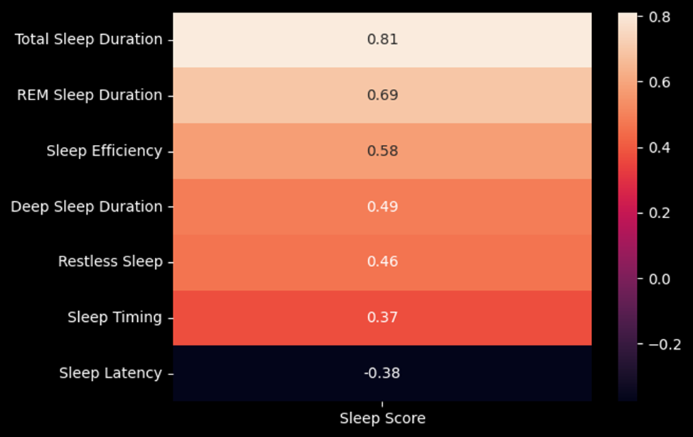
Oura does not expressly state the algorithm used to calculate the sleep score but does note the seven factors that are contributors: Total Sleep, Efficiency, Restfulness, REM Sleep, Deep Sleep, Latency, and Timing.

I used a correlation matrix to see how these factors relate to the Sleep Score using my data. The most strongly correlated values were the Total Sleep Duration and the REM Sleep Duration. Sleep Timing and Sleep Latency show the least correlation to the Sleep Score. Sleep Latency is the only factor that is negatively correlated. Latency means the amount of time it takes to fall asleep. If the latency is larger, your quality of sleep is lower.

From here, I chose to use a Linear Regression model to see how well it could predict the Sleep Score based off of these factors. I started by importing the necessary packages for this modeling.

import numpy as np

import pandas as pd

import matplotlib.pyplot as plt

import math

from sklearn.model_selection import train_test_split

from sklearn.pipeline import Pipeline

from sklearn.preprocessing import StandardScaler

from sklearn.linear_model import LinearRegression

from sklearn.metrics import mean_squared_error, mean_absolute_error, r2_score

At this point, I split the data into the features (X) and the target (y). I then created the training and testing sets, using 80% of the data for training and 20% for testing.

X = data[['Sleep Latency', 'Restless Sleep', 'Sleep Timing', 'REM Sleep Duration', 'Deep Sleep Duration', 'Sleep Efficiency', 'Total Sleep Duration']]

y = data['Sleep Score']

X_train, X_test, y_train, y_test = train_test_split(X, y, test_size = 0.2, random_state=42)

Creating a pipeline is a clean and organized way to make the steps of a model into a single object. The pipeline can then be fit to the training data. The StandardScaler is used to ensure the features have a similar scale. The coefficients found are applied to the features to find the predicted values.

pipeline = Pipeline([('scaler', StandardScaler()),('regression', LinearRegression())])

pipeline.fit(X_train, y_train)

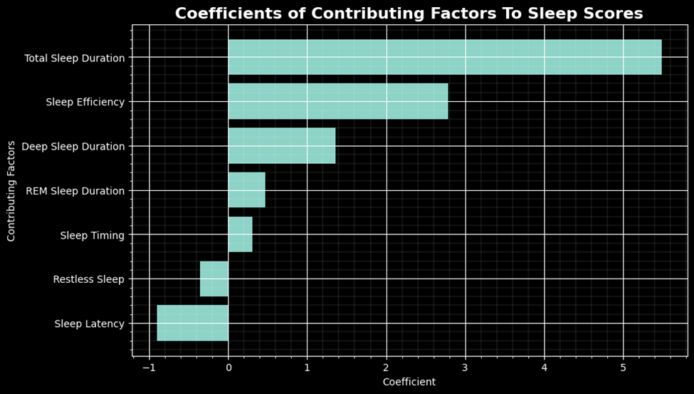
coefficients = pipeline.named_steps['regression'].coef_

intercept = pipeline.named_steps['regression'].intercept_

features = ['Sleep Latency', 'Restless Sleep', 'Sleep Timing', 'REM Sleep Duration', 'Deep Sleep Duration', 'Sleep Efficiency', 'Total Sleep Duration']

plt.figure(figsize=(10, 6))

plt.barh(features, coefficients)

plt.xlabel('Coefficient')

plt.ylabel('Contributing Factors')

plt.title('Coefficients of Contributing Factors To Sleep Scores', fontsize=16, fontweight='bold')

plt.grid(True)

plt.grid(which='minor', linewidth=0.1)

plt.minorticks_on()

plt.show()

The equation used to determine the predicted values is:

y =

84.67

+ (-0.90 * Sleep Latency)

+ (-0.35 * Restless Sleep)

+ (0.31 * Sleep Timing)

+ (0.47 * REM Sleep Duration)

+ (1.36 * Deep Sleep Duration)

+ (2.79 * Sleep Efficiency)

+ (5.49 * Total Sleep Duration)

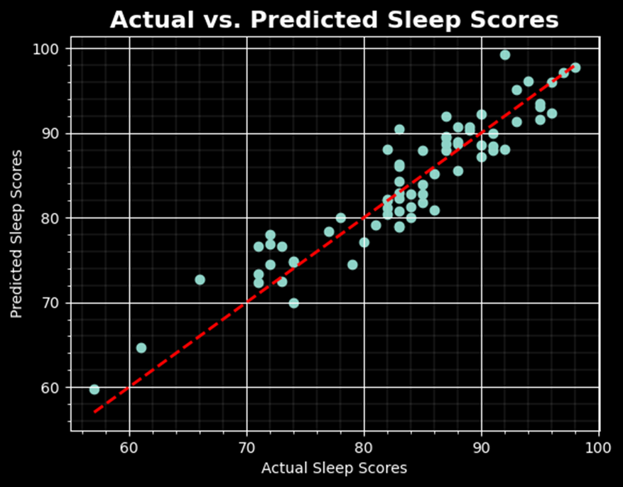
Plotting the predicted values against the actual values, as shown below, indicates generally how well this model performs.

predictions = pipeline.predict(X_test)

plt.scatter(y_test, predictions)

plt.plot([y_test.min(), y_test.max()], [y_test.min(), y_test.max()], 'r--', lw=2)

plt.xlabel('Actual Sleep Scores')

plt.ylabel('Predicted Sleep Scores')

plt.title('Actual vs. Predicted Sleep Scores', fontsize=16, fontweight='bold')

plt.grid(True)

plt.grid(which='minor', linewidth=0.1)

plt.minorticks_on()

plt.show()

The model performance can be evaluated using the Mean Squared Error, Mean Absolute Error, and the R-Squared values.

mse = mean_squared_error(y_test, predictions)

mae = mean_absolute_error(y_test, predictions)

r_squared = r2_score(y_test, predictions)

The results are as follows:

· Mean Squared Error (MSE): 9.5182

· Mean Absolute Error (MAE): 2.5389

· R-squared: 0.8662

An R-squared close to 1 indicates a good model, anything above 0.8 is generally considered to be a strong model.

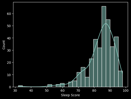
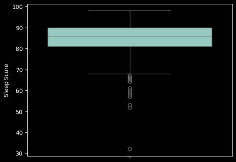
The distribution is left skewed and has several outliers. MSE is preferred for skewed data and is sensitive to outliers and the MAE is less sensitive to outliers. I will use the MSE as the preferred metric for this project. Based on the MSE, the current model can predict within about 3 points the Sleep Score for the night given the seven factors provided which is within reason.

Conclusions

The model may not be exact to what Oura uses to calculate the Sleep Score but it is fairly close. From my dashboard I have gained some insights into what affects my sleep and I look forward to continuing this journey.